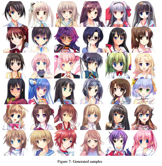
Generative Adversarial Networks are exactly the same thrilling thing. They create some new data out of nothing, following the rules established by existing data. This ability to generate information out of nothing makes GANs look like a bit magical. And the results that are generated are very promising. Yann LeCun — one of the most prominent researchers in deep learning described it as “ the most interesting idea in the last 10 years in Machine Learning”. And indeed GANs have had a huge success and thousands of research papers were published in the recent years.
When you create something out of nothing, it is the most thrilling thing — Frankie Knuckles, American DJ

The main motto of GAN is to generate some information from scratch. But their potential is very huge. Just to give you the idea of their potential, I am mentioning some of the coolest projects created with GANs that you should definitely check out:


So what are Generative Adversarial Networks? What is so magical about them? In this blog post we’ll explore GANs and detailed explanation of how GANs work. But before diving into GANs, we will start by describing what are Generative models.
What is a Generative model?
To understand what a generative model is, contrasting it with a discriminative model is helpful. Discriminative model discriminates between different kinds of data instances whereas a Generative model generates a new data instance. Given the features of a data instance, discriminative model predicts a category to which that data belongs whereas a generative model do the opposite. Instead of predicting a label based on features, a generative model predicts features based on labels. It cares about the distribution of the training data. A Generative Model is a unsupervised learning method that learns any kind of data distribution and it has achieved huge success in the past few years.
Types of Generative models:

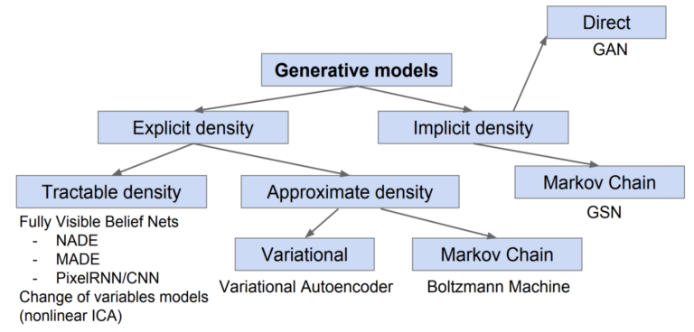
Generative models are of two types — explicit density models and implicit density models. The main difference between them is that explicit models use an explicit density function whereas the implicit models use a stochastic procedure that can directly generate data.
Explicit density models
Explicit density models are again divided into Tractable density and Approximate density models. In general, tractable distribution means it takes polynomial-time to capture probability of its distribution at any given point. Pixel RNN is the most commonly used tractable density model. They are highly effective but they follow sequential generation, which is very slow.
But most of the distributions are complex and it is very difficult to capture the distribution in polynomial time. Such models are considered as Approximate models. These are again divided into two categories: models using variational methods and models using Monte Carlo methods. Variational methods use deterministic approximations and are used in complex models with unknown parameters. Variational Autoencoder (VAE) is one of the most popular generative models and is based on variational learning. Boltzmann machines are another kind of generative models that rely on Markov chains. They use stochastic approximations instead of deterministic approach. Boltzmann machines played an important part in deep learning research but now they are very rarely used because Markov chains inflict very high computational costs.
Implicit density models
These can be trained without explicitly defining a density function. There are some implicit models too which rely on Markov chains like Generative Stochastic Network (GSN) but as we already discussed that Markov chains inflict high computational costs, they fail in many cases. Generative Adversarial Networks were designed to avoid most of these disadvantages associated with other generative models. GANs have become so popular because they are proven to be really successful in modeling and generating high dimensional data.
Enough of this background knowledge. Though it is a very captivating field to explore and discuss, I’ll try to leave the in-depth explanation later in another post, we are here for GANs! Now without wasting any further time, let’s understand how do GANs work !!!
Understanding a GAN
The end goal of a generative model is to predict features given a label, instead of predicting a label given features. They try to learn the model to generate the input distribution as realistic as possible. So the main focus here is to design an architecture of a network that takes a simple N dimensional uniform random variable as input and returns another N dimensional random variable that should somehow follow the probability distribution of input sample as output. Now we need to optimize the network through training. In general, the generated random distribution is directly compared to the input sample and use back propagation to lower the distance between true and generated samples.
Ian Goodfellow and his colleagues came up with a brilliant idea in the 2014 paper titled “Generative Adversarial Nets”. They proposed a new framework in which two neural networks compete with each other for estimating generative models. In the following sections we will understand the training process and the math behind GANs.
The GAN architecture:

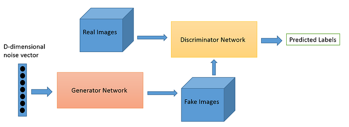
A generative neural network is composed of two models: the Generator which generates data from some random uniform distribution and the Discriminator which identifies the fake data from the real data . The output of generator(fake data) is connected to the discriminator input.
The simplest way to understand the architecture is — a generator network trained to generate samples as realistic as possible via adversarial training by introducing a discriminator network, which plays a role of detecting whether the given sample is real or fake. The generator should learn to fool the discriminator into believing that the input sent by generator is real. While the discriminator tries not to get fooled by generator identifying that the data generated is fake. These two models improves their knowledge by competing with each other, until generator wins in fooling the discriminator.
Since we got an overview of GAN architecture, we will now understand how these models compete with each other technically!
Training a GAN:
We define a neural network G(z, θg) that maps random noise variables z to some data x. We also define another neural network D(x, θd) that outputs a single scalar D(x) that represents the probability that the input came from the real dataset. θg and θd represents parameters that define respective neural networks. The generator and the discriminator have two separate training processes.
The discriminator is simply a classifier. We can use any architecture for the discriminator that is appropriate to the type of data we are using. The discriminator is trained in such a way that it classifies the input data as either real or fake. So the parameters (θd) of the discriminator are updated in order to minimize the probability that any fake data sample G(z) is classified as a real one and also to maximize the probability any real data sample x is classified as belonging to the real dataset. In order words, the loss function of discriminator minimizes D(G(z)) and maximizes D(x). Minimizing log(D(G(z))) is same as maximizing log(1-D(G(z))). So the objective for the discriminator becomes:

The generator learns to make the discriminator classify the data generated as real through feedback from the discriminator. The parameters (θg) of the generator are updated in order to maximize the probability that any fake data sample is classified as a real one. So the loss function of generator maximizes D(G(z)).

As Ian Goodfellow said, it is essentially two-player minimax game played by generator(G) and discriminator(D). The value function V(G, D) is given by:

where —
D(x) : probability that the real data instance x is real
G(z) : generator’s output for noise z
D(G(z)) : probability that the generated instance is real
1-D(G(z)) : probability that the generated instance is fake
A gradient-based optimization algorithm can be used to train the GAN since both the models are neural networks. We perform back propagation which allows the discriminator and generator to improve over time. Based on the classification done by the discriminator we will either have positive or negative feedback in the form of loss gradients. We keep the parameters of generator constant and train the discriminator during which it has to learn how to slap the generator’s flaws. Then we switch the models. We keep the parameters of the discriminator constant and train the generator.
In this way, we train both the networks alternatively and the networks will compete with each other to improve themselves. Eventually the generator generates realistic data and the discriminator will be unable to find the difference between the real data sample and the generated data sample.
I am adding a screenshot from the paper which explains the algorithm on how to train a GAN using stochastic gradient descent.

The training steps for a GAN can be described like this:
- From a random distribution we take some noise and send it to the generator G which produces some generated fake data.
- Along with the generated data, we also send the sample of real data to the discriminator D.
- The discriminator calculates the loss for both the real and fake data samples and the generator also calculates the loss from the noise.
- The two calculated losses are back propagated to their respective networks and the networks learn to improve from these losses.
- Apply optimization algorithm like gradient descent and Repeat the whole process.
“Talk is cheap, Show me the code” — Linus Torvalds
Okay, We’ll now implement a GAN to understand this better.
Implementing a GAN
We are going to implement a GAN using PyTorch. We’ll start by creating a notebook and importing the following dependencies.
import torch
import torch.optim as opt
import torch.nn as nn
import torch.nn.functional as F
import torchvision
import torchvision.transforms as transforms
import numpy as np
Dataset
The Dataset we will be using is the classic MNIST dataset created by LeCunn. The dataset consists of 60,000 images of handwritten digits, each with size 28x28
transform = transforms.ToTensor()
# load data
trainData = torchvision.datasets.MNIST('./data/', download=True, transform=transform, train=True)
# creating a loader with data - which helps to iterate over the data
batch_size = 64
trainLoader = torch.utils.data.DataLoader(trainData, shuffle=True, batch_size=batch_size
Discriminator
This network will take an image as its input and return the probability of it belonging to the real dataset or the generated dataset. The input size for each image will be 28x28=784 . The architecture we are going to implement will have three Fully-connected layers, each followed by ReLU non-linearity layer. Since the output should be the probability of the image that says whether it is real or fake, the value should be between (0,1). For this purpose, a Sigmoid function is added to the real-valued output in the last layer.
class Discriminator(nn.Module):
    def __init__(self):
        super().__init__()
        self.model = nn.Sequential(
            nn.Linear(X_dim, 256),
            nn.LeakyReLU(inplace=True),
            nn.Linear(256,128),
            nn.LeakyReLU(inplace=True),
            nn.Linear(128, 1),
            nn.Sigmoid()
        )

    def forward(self, input):
        return self.model(input)
Generator
The Generator network will take a random noise vector as input and returns a vector of size 784, which resembles a 28x28 image. The last layer will have Tanh activation to clip the image to be [-1,1] — which is same size as the preprocessed MNIST images are bounded.
class Generator(nn.Module):
    def __init__(self):
        super().__init__()
        self.model = nn.Sequential(
            nn.Linear(n_features, 128),
            nn.LeakyReLU(inplace=True),
            nn.Linear(128, 256),
            nn.LeakyReLU(inplace=True),
            nn.Linear(256, X_dim),
            nn.Tanh()
        )

    def forward(self, input):
        return self.model(input)
Optimization
We’ll use Adam as the optimization algorithm with the learning rate 2e-4 which is not necessarily the optimal value, but selected after various tests.
g_opt = opt.Adam(G.parameters(), lr=2e-4)
d_opt = opt.Adam(D.parameters(), lr=2e-4)
Training:
In the above section, we’ve already seen the steps that must be followed to train a GAN. First, we need to calculate losses of both generator and discriminator networks and then back-propagate them.
Discriminator loss function:

Generator loss function:

We will be using Binary Cross Entropy Loss or log loss because it resembles both the generator and the discriminator losses.

For training discriminator, if we replace ŷi with D(x) and yi = 1 we will get the real image loss and if we replace ŷi with D(G(z)) and yi = 0 we will get fake image loss. We will add this together to get the total discriminator loss.
For training generator, we need to minimize log(1 - D(G(z))) which is same as maximizing log(D(G(z))). If we replace ŷi with D(G(z)) and yi = 1, we will get the loss to be maximized. But the problem with most of the frameworks like PyTorch is — they minimize the functions. Since, BCE-loss definition has a minus-sign, this won’t cause us any problem.
We will also create the real-image targets as ones, and the fake-image targets as zeros with shape (batch_size, 1). These will be help us in calculating the losses of generator and discriminator.
Training loop:
for epoch in range(20):
    G_loss_update = 0.0
    D_loss_update = 0.0
    for i, data in enumerate(trainLoader):
        X, _ = data
        X = X.view(X.size(0), -1)
        batch_size = X.size(0)

        # tensor containing ones representing real data target
        real_target = torch.ones(batch_size, 1)
        # tensor containing zeroes representing generated data target
        generated_target = torch.zeros(batch_size, 1)

        z = torch.randn(batch_size, n_features)

        # 1. Train discriminator
        # on real data
        D_real = D(X)
        # calculating real data error
        D_real_loss = F.binary_cross_entropy(D_real, real_target)

        # on generated data
        D_generated = D(G(z))
        # calculating generated data error
        D_generated_loss = F.binary_cross_entropy(D_generated, generated_target)

        # Total discriminator loss
        D_loss = D_real_loss + D_generated_loss

        # reset gradients
        d_opt.zero_grad()
        # backpropagate
        D_loss.backward()
        # update weights with gradients
        d_opt.step()

        # 2. Train generator
        # sample noise and generate some fake data
        z = torch.randn(batch_size, n_features)
        D_generated = D(G(z))
        # calculating error
        G_loss = F.binary_cross_entropy(D_generated, real_target)

        # resetting gradients, backpropagating and updating weights
        g_opt.zero_grad()
        G_loss.backward()
        g_opt.step()

        G_loss_update = G_loss_update + G_loss.item()
        D_loss_update = D_loss_update + D_loss.item()

    print('Epoch:{}, G_loss:{}, D_loss:{}'.format(epoch, G_loss_update/(i+1), D_loss_update/(i+1)))

    samples = G(z).detach()
    samples = samples.view(samples.size(0), 1, 28, 28).cpu()
    imshow(samples)
We have successfully implemented a GAN. Now, let’s look at the results -
Before training:

During training at 10th epoch:

Finally:

You can check out the complete implementation and run it online — kaggle notebook
References:
[1] Goodfellow, Ian, et al. “Generative Adversarial Networks” NIPS, 2014.
[2] Uddin, S. M. Nadim. (2019). Intuitive Approach to Understand the Mathematics Behind GAN. 10.13140/RG.2.2.12650.36805.
[3] Ian Goodfellow’s NIPS 2016 tutorial on YouTube.